Its a very frequent requirement to transform data in your excel sheet to meet some of your requirement or understanding. Today, we are going to see how we can transform data (unpivot) using Power Query in Excel.

Steps to transform/unpivot data in Excel

Select the data range to be considered -> Click “From Table/Range” under “Data” Menu.

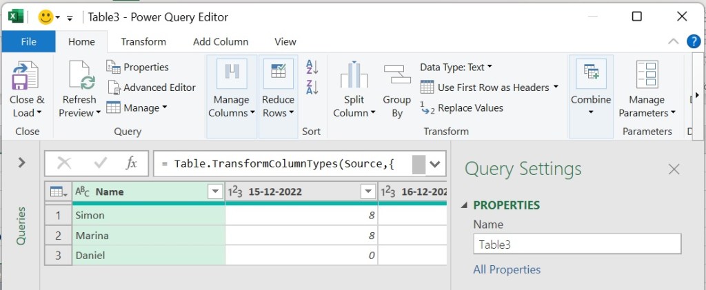
It will open a new Power Query window as below.

Right Click on “First Column – Name” and select “UnPivot Other Columns”

Rename the column names as required in the Query Editor

Finally, “Close & Load” the query window which will open a new Table sheet

If you enjoyed this blog post, please share it with your friends!